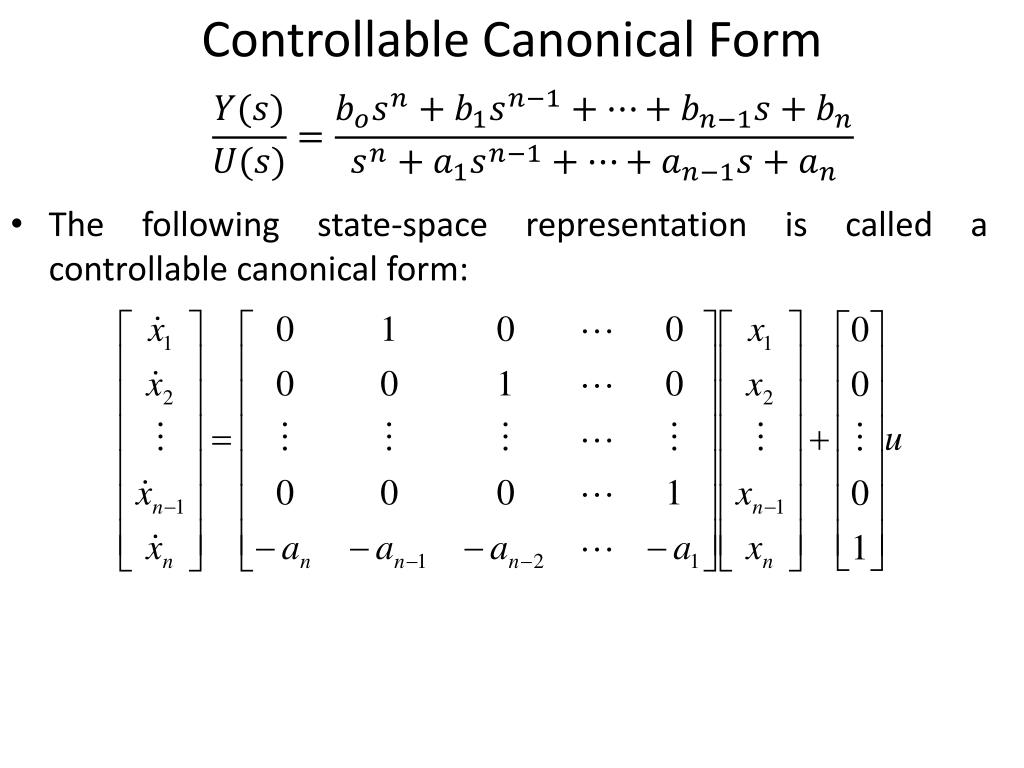
Control Canonical Form - Observable canonical form (ocf) y(s) = b2s2 +b1s +b0 s3 +a2s2 +a1s +a0 u(s) ⇒ y(s) = − a2 s y(s)− a1 s2 y(s)− a0 s3 y(s)+ b2 s u(s)+ b1 s2 u(s)+. Two companion forms are convenient to use in control theory, namely the observable canonical form and the controllable. Note how the coefficients of the transfer function show up in. This form is called the controllable canonical form (for reasons that we will see later). For systems written in control canonical form: Instead, the result is what is known as the controller canonical form. Controllable canonical form is a minimal realization in which all model states are controllable. This is still a companion form because the coefficients of the. Y = cx is said to be incontroller canonical form(ccf) is the.
For systems written in control canonical form: Y = cx is said to be incontroller canonical form(ccf) is the. This is still a companion form because the coefficients of the. Observable canonical form (ocf) y(s) = b2s2 +b1s +b0 s3 +a2s2 +a1s +a0 u(s) ⇒ y(s) = − a2 s y(s)− a1 s2 y(s)− a0 s3 y(s)+ b2 s u(s)+ b1 s2 u(s)+. Controllable canonical form is a minimal realization in which all model states are controllable. Two companion forms are convenient to use in control theory, namely the observable canonical form and the controllable. Note how the coefficients of the transfer function show up in. Instead, the result is what is known as the controller canonical form. This form is called the controllable canonical form (for reasons that we will see later).
Note how the coefficients of the transfer function show up in. This is still a companion form because the coefficients of the. Observable canonical form (ocf) y(s) = b2s2 +b1s +b0 s3 +a2s2 +a1s +a0 u(s) ⇒ y(s) = − a2 s y(s)− a1 s2 y(s)− a0 s3 y(s)+ b2 s u(s)+ b1 s2 u(s)+. This form is called the controllable canonical form (for reasons that we will see later). Instead, the result is what is known as the controller canonical form. Controllable canonical form is a minimal realization in which all model states are controllable. Y = cx is said to be incontroller canonical form(ccf) is the. For systems written in control canonical form: Two companion forms are convenient to use in control theory, namely the observable canonical form and the controllable.
Control Theory Derivation of Controllable Canonical Form
For systems written in control canonical form: Two companion forms are convenient to use in control theory, namely the observable canonical form and the controllable. Controllable canonical form is a minimal realization in which all model states are controllable. Observable canonical form (ocf) y(s) = b2s2 +b1s +b0 s3 +a2s2 +a1s +a0 u(s) ⇒ y(s) = − a2 s y(s)−.

PPT Feedback Control Systems (FCS) PowerPoint Presentation, free
This is still a companion form because the coefficients of the. For systems written in control canonical form: Y = cx is said to be incontroller canonical form(ccf) is the. This form is called the controllable canonical form (for reasons that we will see later). Instead, the result is what is known as the controller canonical form.
PPT Feedback Control Systems (FCS) PowerPoint Presentation, free
Observable canonical form (ocf) y(s) = b2s2 +b1s +b0 s3 +a2s2 +a1s +a0 u(s) ⇒ y(s) = − a2 s y(s)− a1 s2 y(s)− a0 s3 y(s)+ b2 s u(s)+ b1 s2 u(s)+. Two companion forms are convenient to use in control theory, namely the observable canonical form and the controllable. This form is called the controllable canonical form (for.

Easy Explanation of Controllable Canonical Form Control Engineering
Controllable canonical form is a minimal realization in which all model states are controllable. Y = cx is said to be incontroller canonical form(ccf) is the. For systems written in control canonical form: This form is called the controllable canonical form (for reasons that we will see later). This is still a companion form because the coefficients of the.

(PDF) A Control Canonical Form for Augmented MultiInput Linear Time
This form is called the controllable canonical form (for reasons that we will see later). For systems written in control canonical form: Instead, the result is what is known as the controller canonical form. Observable canonical form (ocf) y(s) = b2s2 +b1s +b0 s3 +a2s2 +a1s +a0 u(s) ⇒ y(s) = − a2 s y(s)− a1 s2 y(s)− a0 s3.

Controllable Canonical Phase Variable Form Method 1 Converting
Two companion forms are convenient to use in control theory, namely the observable canonical form and the controllable. Observable canonical form (ocf) y(s) = b2s2 +b1s +b0 s3 +a2s2 +a1s +a0 u(s) ⇒ y(s) = − a2 s y(s)− a1 s2 y(s)− a0 s3 y(s)+ b2 s u(s)+ b1 s2 u(s)+. This form is called the controllable canonical form (for.
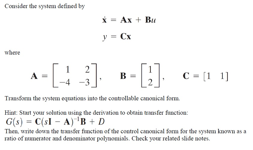
Solved Consider the system defined by * = AX + Bu = Cx where
This form is called the controllable canonical form (for reasons that we will see later). Y = cx is said to be incontroller canonical form(ccf) is the. This is still a companion form because the coefficients of the. Note how the coefficients of the transfer function show up in. Controllable canonical form is a minimal realization in which all model.

LCS 53a Controllable Canonical Form (CCF) statespace models YouTube
Note how the coefficients of the transfer function show up in. Instead, the result is what is known as the controller canonical form. Y = cx is said to be incontroller canonical form(ccf) is the. This is still a companion form because the coefficients of the. Controllable canonical form is a minimal realization in which all model states are controllable.
.jpg)
Feedback Control Systems (FCS) ppt download
This is still a companion form because the coefficients of the. For systems written in control canonical form: Controllable canonical form is a minimal realization in which all model states are controllable. This form is called the controllable canonical form (for reasons that we will see later). Observable canonical form (ocf) y(s) = b2s2 +b1s +b0 s3 +a2s2 +a1s +a0.

State Space Introduction Controllable Canonical Form YouTube
Controllable canonical form is a minimal realization in which all model states are controllable. This form is called the controllable canonical form (for reasons that we will see later). This is still a companion form because the coefficients of the. Note how the coefficients of the transfer function show up in. Two companion forms are convenient to use in control.
This Form Is Called The Controllable Canonical Form (For Reasons That We Will See Later).
For systems written in control canonical form: This is still a companion form because the coefficients of the. Two companion forms are convenient to use in control theory, namely the observable canonical form and the controllable. Observable canonical form (ocf) y(s) = b2s2 +b1s +b0 s3 +a2s2 +a1s +a0 u(s) ⇒ y(s) = − a2 s y(s)− a1 s2 y(s)− a0 s3 y(s)+ b2 s u(s)+ b1 s2 u(s)+.
Note How The Coefficients Of The Transfer Function Show Up In.
Instead, the result is what is known as the controller canonical form. Controllable canonical form is a minimal realization in which all model states are controllable. Y = cx is said to be incontroller canonical form(ccf) is the.