Google Sheets Conditional Format Row Based On Cell - To format an entire row based on the value of one of the cells in that row: And today we will see the conditional. To highlight a row based on a cell value, we need to use the “custom formula is” option in the conditional formatting menu. On your computer, open a spreadsheet in google sheets. Conditional formatting is quite a versatile function in any spreadsheet application.
To highlight a row based on a cell value, we need to use the “custom formula is” option in the conditional formatting menu. To format an entire row based on the value of one of the cells in that row: Conditional formatting is quite a versatile function in any spreadsheet application. And today we will see the conditional. On your computer, open a spreadsheet in google sheets.
And today we will see the conditional. To format an entire row based on the value of one of the cells in that row: To highlight a row based on a cell value, we need to use the “custom formula is” option in the conditional formatting menu. Conditional formatting is quite a versatile function in any spreadsheet application. On your computer, open a spreadsheet in google sheets.

Learn About Google Sheets Conditional Formatting Based on Another Cell
To format an entire row based on the value of one of the cells in that row: And today we will see the conditional. On your computer, open a spreadsheet in google sheets. Conditional formatting is quite a versatile function in any spreadsheet application. To highlight a row based on a cell value, we need to use the “custom formula.
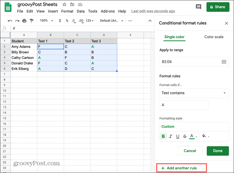
How to Set Up Multiple Conditional Formatting Rules in Google Sheets
On your computer, open a spreadsheet in google sheets. Conditional formatting is quite a versatile function in any spreadsheet application. And today we will see the conditional. To highlight a row based on a cell value, we need to use the “custom formula is” option in the conditional formatting menu. To format an entire row based on the value of.

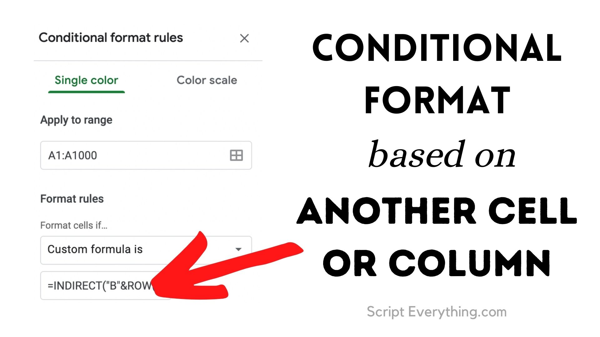
How to Do Conditional Formatting Based On Another Cell in Google Sheets
To highlight a row based on a cell value, we need to use the “custom formula is” option in the conditional formatting menu. On your computer, open a spreadsheet in google sheets. To format an entire row based on the value of one of the cells in that row: And today we will see the conditional. Conditional formatting is quite.

Conditional Row Manipulation Based On Cell Values Excel Template And
And today we will see the conditional. To format an entire row based on the value of one of the cells in that row: To highlight a row based on a cell value, we need to use the “custom formula is” option in the conditional formatting menu. Conditional formatting is quite a versatile function in any spreadsheet application. On your.
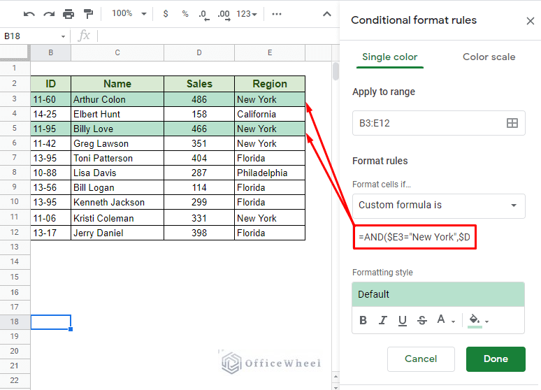
Set Conditional Format Based On Another Cell Value In Google Sheets
Conditional formatting is quite a versatile function in any spreadsheet application. To format an entire row based on the value of one of the cells in that row: And today we will see the conditional. To highlight a row based on a cell value, we need to use the “custom formula is” option in the conditional formatting menu. On your.
Google sheet định dạng có điều kiện thêm văn bản
To format an entire row based on the value of one of the cells in that row: On your computer, open a spreadsheet in google sheets. And today we will see the conditional. To highlight a row based on a cell value, we need to use the “custom formula is” option in the conditional formatting menu. Conditional formatting is quite.

Google Sheets Conditional Formatting with Custom Formula Yagisanatode
To highlight a row based on a cell value, we need to use the “custom formula is” option in the conditional formatting menu. Conditional formatting is quite a versatile function in any spreadsheet application. On your computer, open a spreadsheet in google sheets. To format an entire row based on the value of one of the cells in that row:.
![[Solved] Conditional Formatting Based on Another Cell the Solution](https://assets.anakin.ai/blog/2024/04/image-78.png)
[Solved] Conditional Formatting Based on Another Cell the Solution
And today we will see the conditional. To highlight a row based on a cell value, we need to use the “custom formula is” option in the conditional formatting menu. Conditional formatting is quite a versatile function in any spreadsheet application. To format an entire row based on the value of one of the cells in that row: On your.
Google Sheets Conditional Formatting Row Based on Cell
To highlight a row based on a cell value, we need to use the “custom formula is” option in the conditional formatting menu. Conditional formatting is quite a versatile function in any spreadsheet application. And today we will see the conditional. To format an entire row based on the value of one of the cells in that row: On your.

Conditional Formatting Rows Google Sheets Update
Conditional formatting is quite a versatile function in any spreadsheet application. On your computer, open a spreadsheet in google sheets. To highlight a row based on a cell value, we need to use the “custom formula is” option in the conditional formatting menu. To format an entire row based on the value of one of the cells in that row:.
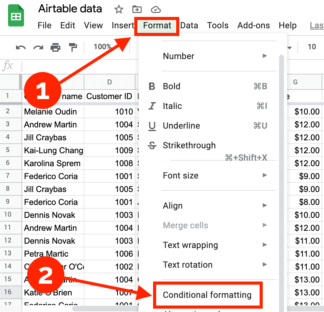
On Your Computer, Open A Spreadsheet In Google Sheets.
Conditional formatting is quite a versatile function in any spreadsheet application. To format an entire row based on the value of one of the cells in that row: And today we will see the conditional. To highlight a row based on a cell value, we need to use the “custom formula is” option in the conditional formatting menu.